The goal of ham is to provide different modeling approaches to evaluating healthcare programs (or programs in other fields) with regression analysis. This includes standard regression methods like linear (OLS) and logistic regression. And ham adds options for differences-in-differences models as well as interrupted time-series analysis. DID and ITS models offer options for causal modeling. What is unique about ham is that it creates datasets with constructed variables for DID and ITS models, optionally it can add top coded outcome variables, propensity scores, and provides some interpretation of model results. Additionally, Cronbach’s alpha can be calculated for such things as patient surveys. As the logo of Dr. Ham suggests, the ham package can help illuminate your results.

You can install the development version of ham from GitHub with:
# install.packages("devtools")
devtools::install_github("szuniga07/ham")An example of calculating Cronbach’s alpha:
library(ham)
alpha(items=c("i1","i2","i3","i4","i5"), data=cas)
#> Scale statistics
#> Cronbach's alpha   = 0.919
#> Mean               = 3.772
#> Variance           = 0.453
#> Standard Deviation = 0.673
#> Items              = 5
#>
#> Item statistics
#>    Mean Variance Std. Dev.
#> i1 3.50    0.434     0.659
#> i2 3.81    0.681     0.825
#> i3 3.88    0.652     0.808
#> i4 3.82    0.594     0.770
#> i5 3.85    0.634     0.796
#>
#> Scale statistics if item deleted
#>    Alpha  Mean Variance Std. Dev.
#> i1 0.930 3.840    0.528     0.727
#> i2 0.891 3.763    0.436     0.660
#> i3 0.883 3.745    0.433     0.658
#> i4 0.910 3.760    0.472     0.687
#> i5 0.885 3.752    0.439     0.662
#>
#> Sample
#> Total    = 100
#> Valid    = 100
#> Excluded = 0

## Interpret the results
interpret(alpha(items=c("i1","i2","i3","i4","i5"), data=cas))
#> Interpretations: Alpha
#> ----------------------
#> Your 5 item scale has a Cronbach's alpha of 0.92. This is
#> generally considered as being in the 'excellent' range.
#>
#> The scale mean is 3.77 and has a standard deviation of 0.67.
#>
#> Removing one of these item(s): i1, can improve the Cronbach's
#> alpha in a new scale to a higher level than the current alpha
#> based on all items.
#>
#> 0 row(s) of data excluded from the analysis because of missing
#> data.This is the ham package on healthcare analysis methods. This package can help when performing program evaluations or intervention studies in healthcare. Or simply to test if a program has an impact on an outcome of interest.
ham can help with research or evaluation studies. When working in healthcare systems, multi-site evaluations can strongly resemble research studies and commonly use regression methods. For an introduction to evaluation, please see the reference below.
Patton, M. Q. (1997). Utilization-focused evaluation: The new century text (3rd ed.). Thousand Oaks, CA: Sage Publications
What is unique about ham, is that it provides options for running standard linear or ordinary least squares (OLS) and logistic regression as well as methods used in causal modeling such as differences-in-differences (DID) and interrupted time series analysis (ITS). It also optionally makes data with the newly created variables (i.e., this saves you time).
This vignette will introduce ham’s features in the following functions: * alpha: Conduct Cronbach’s alpha on scale items (e.g., survey questions). * assess: Perform various regression methods (OLS, logistic, differences-in-differences, and interrupted time series) * importance: Rank variable importance from regression coefficients using the partial chi-square statistic. * interpret: Provides simple coefficient interpretations. This is a helpful reminder, especially as models have increased coefficients (e.g., ITS). * There are also printing and plotting options to help review your results.
Below will cover 3 sections with examples of the different features along the way.
This example shows group level point estimates and confidence intervals. There is also an option to retrieve those estimates over time periods. And there are graphing options to help see how the data looks for both.
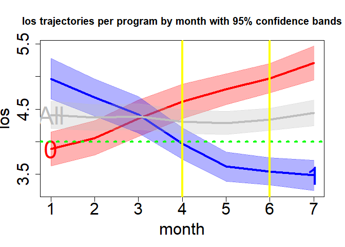
Results can be returned for each unit of time, as increments such as for each 3 months (i.e., quarters) or for rolling averages such as a rolling 12-month period. Using increments of multiple months or as rolling averages can help visualize results when there is high variation over time.
gr1 <- group(x="program", y="los", z="month", dataf=hosprog, dist="t", increment=3, rolling=6)
print(gr1$Group.CI)
#> $adf_alpha
#>   Group PointEst    Lower    Upper
#> 1     1 4.247012 4.034842 4.459181
#> 0     0 4.585967 4.391132 4.780802
#>
#> $adf_numeric
#>   Group PointEst    Lower    Upper
#> 0     0 4.585967 4.391132 4.780802
#> 1     1 4.247012 4.034842 4.459181
#>
#> $adf_all
#>   PointEst    Lower    Upper
#> 1 4.428259 4.284543 4.571974plot(x=gr1, y="group", order="numeric", lwd=4, gcol= "blue", pcol="red", overall=TRUE, oband=TRUE, ocol="gray", tcol="green", tgt=4.5, cex=2, cex.axis=1, cex.lab=1.1, cex.text=2, cex.main=1.25, adj.alpha=.2)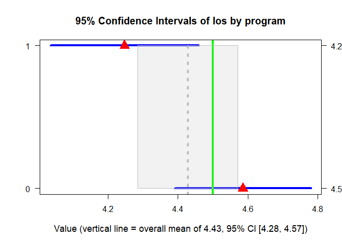
plot(x=gr1, y="time", lwd=4, gcol=c("red", "blue"), gband=TRUE, overall=TRUE, oband=TRUE, ocol="gray", tcol="green", tgt=4, tpline=3, tpcol="yellow", name=TRUE, cex.axis=1, cex.lab=1, cex.text=2, cex.main=1.25, adj.alpha=.3)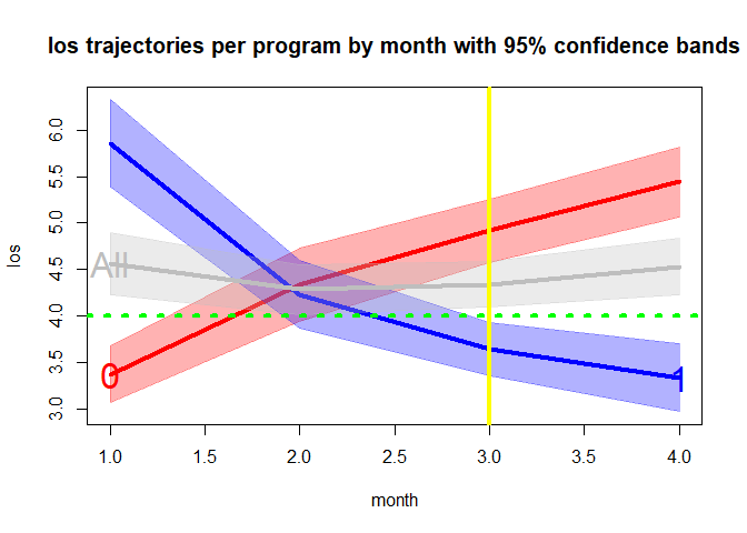
The example dataset has common variables found in program evaluation or intervention studies (I’ll refer to both as a ‘study’), there are various outcome and predictor variables (or response and explanatory variables or dependent and independent variables or other names common in your field). In these studies, we try to assess the impact of the predictors on the outcome. We often use treatment and control groups to asses a healthcare program or intervention’s impact on our key outcome variable of interest. Because of multiple stakeholders, we often conduct these studies with multiple outcomes to help answer the multiple stakeholder’s questions.
A common approach to answering study questions is using a regression to test a treatment effect while controlling for other covariates.
Here are OLS and logistic regression example using assess() on the mtcars data. These use lm() and glm() found in R’s stats package.
summary(assess(hp ~ mpg+wt, data=mtcars, regression="ols")$model)
#>
#> Call:
#> stats::lm(formula = primary_formula, data = combined_df)
#>
#> Residuals:
#>    Min     1Q Median     3Q    Max
#> -59.42 -30.75 -12.07  24.82 141.84
#>
#> Coefficients:
#>             Estimate Std. Error t value Pr(>|t|)
#> (Intercept)  349.287    103.509   3.374  0.00212 **
#> mpg           -9.417      2.676  -3.519  0.00145 **
#> wt            -4.168     16.485  -0.253  0.80217
#> ---
#> Signif. codes:  0 '***' 0.001 '**' 0.01 '*' 0.05 '.' 0.1 ' ' 1
#>
#> Residual standard error: 44.65 on 29 degrees of freedom
#> Multiple R-squared:  0.6033, Adjusted R-squared:  0.576
#> F-statistic: 22.05 on 2 and 29 DF, p-value: 1.505e-06summary(assess(formula=vs~mpg+wt+hp, data=mtcars, regression="logistic")$model)
#>
#> Call:
#> stats::glm(formula = primary_formula, family = binomial(link = "logit"),
#> data = combined_df)
#>
#> Coefficients:
#> Estimate Std. Error z value Pr(>|z|)
#> (Intercept) -10.61945 16.52453 -0.643 0.5205
#> mpg 0.50291 0.48656 1.034 0.3013
#> wt 3.87749 3.19255 1.215 0.2245
#> hp -0.09318 0.04318 -2.158 0.0309 *
#> ---
#> Signif. codes: 0 '***' 0.001 '**' 0.01 '*' 0.05 '.' 0.1 ' ' 1
#>
#> (Dispersion parameter for binomial family taken to be 1)
#>
#> Null deviance: 43.860 on 31 degrees of freedom
#> Residual deviance: 14.748 on 28 degrees of freedom
#> AIC: 22.748
#>
#> Number of Fisher Scoring iterations: 8
## Interpret the results
interpret(assess(formula=vs~mpg+wt+hp, data=mtcars, regression="logistic")
)$model
#> Interpretations: Model
#> ----------------------
#> These estimates tell you about the relationship between the
#> independent variables and the dependent variable. These estimates
#> tell the amount of change in outcome scores that would be
#> predicted by a 1 unit increase in the predictor.
#>
#> The following predictor variable(s) have coefficient(s)
#> significantly different from 0 using an alpha of 0.05:
#> hp
#>
#> For every 1 unit increase in these predictor variables,
#> vs is predicted to increase by the value of the
#> coefficient, holding all other variables constant. The following
#> predictor variable(s) have positive coefficient(s) that
#> increase the predicted value of the outcome:
#> No positive coefficients in your model were significant.
#>
#> For every 1 unit increase in these predictor variables,
#> vs is predicted to decrease by the value of the
#> coefficient, holding all other variables constant. The following
#> predictor variable(s) have negative coefficient(s) that
#> decrease the predicted value of the outcome:
#> hp
#>
#> There is no R2 information provided.ham can topcode the outcome and create a propensity score variable. Here is an example using the artificially created hosprog data with hospital stay cost as the outcome with a novel hospital program/intervention binary indicator and a 12 month time variable. The option for new data being returned is specified with newdata=TRUE.
top coding cost at $17,150 and propensity score based on age, female indicator, and a health risk probability score.
m1 <- assess(formula=cost ~ month * program, data=hosprog, intervention = "program",
regression="ols", topcode=17150, propensity=c("female","age","risk"),
newdata=TRUE)summary(m1$model)
#>
#> Call:
#> stats::lm(formula = primary_formula, data = combined_df)
#>
#> Residuals:
#> Min 1Q Median 3Q Max
#> -6570.9 -2158.3 -598.1 1962.0 10521.1
#>
#> Coefficients:
#> Estimate Std. Error t value Pr(>|t|)
#> (Intercept) 14006.64 1363.65 10.271 < 2e-16 ***
#> month 424.81 46.57 9.122 < 2e-16 ***
#> program 5524.74 514.18 10.745 < 2e-16 ***
#> pscore -15989.00 2838.57 -5.633 2.55e-08 ***
#> month:program -908.68 68.64 -13.239 < 2e-16 ***
#> ---
#> Signif. codes: 0 '***' 0.001 '**' 0.01 '*' 0.05 '.' 0.1 ' ' 1
#>
#> Residual standard error: 3165 on 715 degrees of freedom
#> Multiple R-squared: 0.233, Adjusted R-squared: 0.2287
#> F-statistic: 54.3 on 4 and 715 DF, p-value: < 2.2e-16Descriptive statistics on newly created variables and the original cost as a comparison. top.cost is the topcoded cost variable.
summary(m1$newdata[, c( "cost","top.cost", "pscore")])
#>       cost          top.cost         pscore
#>  Min.   : 1483   Min.   : 1483   Min.   :0.3708
#>  1st Qu.: 6410   1st Qu.: 6410   1st Qu.:0.4364
#>  Median : 8639   Median : 8639   Median :0.4655
#>  Mean   : 9348   Mean   : 9215   Mean   :0.4653
#>  3rd Qu.:11487   3rd Qu.:11487   3rd Qu.:0.4942
#> Max. :27540 Max. :17150 Max. :0.5609We can examine variable importance based on partial chi-square (i.e., which variables explain the outcome the most).
importance(m1$model)
#>               X    Chi.Sq d.f.      p.value
#> 1         month 175.30630    2 8.564878e-39
#> 2       program 179.92844    2 8.492485e-40
#> 3        pscore  31.72813    1 1.773352e-08
#> 4 month:program 175.27159 1 5.222734e-40We can examine variable importance to see a ranking of variables with a graph. The hospital program has the highest rank, variables highlighted in red are statistically significant.
#Consider using these graphical parameters
par(mar=c(4.2, 2, 3.5, 3))
par(oma = c(0, 0, 0, 3))
plot(importance(m1$model))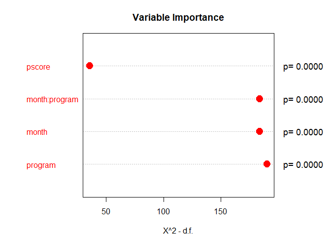
Topcoding can be applied to any model. Propensity scores can be created for any model except the single group interrupted time series because there is no control group (i.e. intervention group only).
DID can be used on binary or continuous outcome variables. Below is an example using the hosprog data with length of stay as the outcome and the created DID variables as the predictors, use ‘.’ on the right-hand side of the formula to indicate only the created variables will be used. Replace ‘.’ with any additional selected variables. The newly created DID variables will be added in all DID models. This model has a pre/post design (i.e., there are only 2 distinct time points) by selecting: did=“two”, with post starting at month 5.
dm1 <- assess(formula= los ~ ., data=hosprog, intervention = "program",
int.time="month", treatment= 5, did="two")summary(dm1$DID)
#>
#> Call:
#> stats::lm(formula = DID_formula, data = combined_df)
#>
#> Residuals:
#> Min 1Q Median 3Q Max
#> -3.6247 -1.2003 -0.3145 0.8564 8.8642
#>
#> Coefficients:
#> Estimate Std. Error t value Pr(>|t|)
#> (Intercept) 3.4940 0.1650 21.175 < 2e-16 ***
#> Post.All 1.5629 0.1974 7.917 9.25e-15 ***
#> Int.Var 2.0664 0.2349 8.797 < 2e-16 ***
#> DID -3.5448 0.2849 -12.444 < 2e-16 ***
#> ---
#> Signif. codes: 0 '***' 0.001 '**' 0.01 '*' 0.05 '.' 0.1 ' ' 1
#>
#> Residual standard error: 1.777 on 716 degrees of freedom
#> Multiple R-squared: 0.1848, Adjusted R-squared: 0.1814
#> F-statistic: 54.11 on 3 and 716 DF, p-value: < 2.2e-16interpret(dm1)$did
#> Interpretations: DID
#> --------------------
#> The intercept represents the mean los value of the
#> control group at the baseline period (Time 1): 3.494.
#>
#> Post.All is the change in the control group's los
#> value in the 2nd time period (Time 2). There was a
#> significant increase for the control group
#> at time 2: 1.563.
#>
#> Int.Var is the difference between the intervention
#> and control group at the baseline period (Time 1). The
#> intervention group had a significant increase in the
#> mean los value compared to the control group: 2.066.
#>
#> DID estimates the average treatment effect on the
#> treated group (ATET). This interaction represents the
#> difference in the trend differences for the intervention and
#> control groups:
#> (Int. Time 2 - Int. Time 1) - (Ctl. Time 2 - Ctl. Time 1) = -3.545.
#> In other words, there was a significant decrease in the
#> mean los trend by -3.545 for the intervention group.
#>
#> If there are additional variables in the model then the coefficients
#> above represent the effects after controlling for the other variables.This model allows for more than 2 time points. It allows for monthly increments by selecting did=“many”.
dm2 <- assess(formula= los ~ ., data=hosprog, intervention = "program",
int.time="month", treatment= 5, did="many")summary(dm2$DID)
#>
#> Call:
#> stats::lm(formula = DID_formula, data = combined_df)
#>
#> Residuals:
#> Min 1Q Median 3Q Max
#> -3.7149 -1.2747 -0.3732 0.8838 9.1718
#>
#> Coefficients:
#> Estimate Std. Error t value Pr(>|t|)
#> (Intercept) 4.17164 0.16049 25.994 < 2e-16 ***
#> Period 0.10837 0.02342 4.627 4.4e-06 ***
#> DID 0.14843 0.48630 0.305 0.760284
#> DID.Trend -0.19580 0.05712 -3.428 0.000643 ***
#> ---
#> Signif. codes: 0 '***' 0.001 '**' 0.01 '*' 0.05 '.' 0.1 ' ' 1
#>
#> Residual standard error: 1.853 on 716 degrees of freedom
#> Multiple R-squared: 0.1135, Adjusted R-squared: 0.1098
#> F-statistic: 30.57 on 3 and 716 DF, p-value: < 2.2e-16interpret(dm2)$did
#> Interpretations: DID
#> --------------------
#> The intercept represents the starting point of the control
#> group's trend line at the baseline period (Time 1): 4.172.
#>
#> Period is the change in the control group's los value trend
#> line after the baseline period. There was a significant increase
#> for the control group after the baseline period: 0.108.
#>
#> DID estimates the difference in mean overall level between
#> the intervention and both the non-intervention period/group.
#> In other words, there was a non-significant increase in the
#> mean los by 0.148 for the intervention group.
#>
#> DID.Trend is the difference in the intervention group's
#> trend line after the intervention period started (> Time 1).
#> The intervention group had a significant decrease in trend
#> of the mean los by -0.196 after the intervention started.
#>
#> If there are additional variables in the model then the coefficients
#> above represent the effects after controlling for the other variables.We can also use DID on binary outcomes like hospital re-admission within 30-days.
dm3 <- assess(formula= rdm30 ~ ., data=hosprog, intervention = "program",
int.time="month", treatment= 5, did="two")summary(dm3$DID)
#>
#> Call:
#> stats::lm(formula = DID_formula, data = combined_df)
#>
#> Residuals:
#> Min 1Q Median 3Q Max
#> -0.31858 -0.25651 -0.07207 -0.06034 0.93966
#>
#> Coefficients:
#> Estimate Std. Error t value Pr(>|t|)
#> (Intercept) 0.06034 0.03422 1.763 0.0782 .
#> Post.All 0.19616 0.04094 4.792 2.01e-06 ***
#> Int.Var 0.25824 0.04871 5.301 1.53e-07 ***
#> DID -0.44267 0.05907 -7.493 1.98e-13 ***
#> ---
#> Signif. codes: 0 '***' 0.001 '**' 0.01 '*' 0.05 '.' 0.1 ' ' 1
#>
#> Residual standard error: 0.3686 on 716 degrees of freedom
#> Multiple R-squared: 0.0759, Adjusted R-squared: 0.07203
#> F-statistic: 19.6 on 3 and 716 DF, p-value: 3.197e-12Significant DID effect showing reduced re-admissions
ITS lets us look at trends for 1 or 2 groups such as an intervention/treatment group without a control group or both a treatment and control group. And we have the option of one or more treatment periods (or interruptions). This gives us 4 options that can be specified using the interrupt and its= arguments.
Below are examples using the hosprog data for the patient length of stay (LOS) and death within 30-days. The dataset hosp1 will be used for the single group examples.
We begin by looking at a single group with a single interruption/treatment period and assessing their LOS scores. We specify it with: interrupt= 5 and its=“one”.
im11 <- assess(formula=los ~ ., data=hosp1, intervention = "program",
int.time="month", interrupt= 5, its="one")summary(im11$ITS)
#>
#> Call:
#> stats::lm(formula = ITS_formula, data = combined_df)
#>
#> Residuals:
#> Min 1Q Median 3Q Max
#> -3.7673 -1.1321 -0.3755 0.5758 9.1718
#>
#> Coefficients:
#> Estimate Std. Error t value Pr(>|t|)
#> (Intercept) 6.3299 0.4170 15.178 <2e-16 ***
#> ITS.Time -0.2889 0.1442 -2.003 0.0460 *
#> post5 -1.0026 0.4264 -2.351 0.0193 *
#> txp5 0.2014 0.1522 1.324 0.1865
#> ---
#> Signif. codes: 0 '***' 0.001 '**' 0.01 '*' 0.05 '.' 0.1 ' ' 1
#>
#> Residual standard error: 1.726 on 331 degrees of freedom
#> Multiple R-squared: 0.2426, Adjusted R-squared: 0.2357
#> F-statistic: 35.34 on 3 and 331 DF, p-value: < 2.2e-16interpret(im11)$its
#> Interpretations: ITS
#> --------------------
#> Note: Some variable names below based on time points (or 'interruptions').
#> This analysis is for a one-group, single intervention period (interruption).
#>
#> Intercept is 6.33 and the starting value of the trend
#> for the intervention group.
#>
#> ITS.Time is -0.289 and the slope prior to intervention.
#> The coefficient is significant.
#>
#> post5 is -1.003 and the immediate shift in the trend line
#> after the intervention start (e.g., 1st year of intervention).
#> The coefficient is significant.
#>
#> txp5 is 0.201 and the difference between pre- and
#> post-intervention slopes (e.g., change in the pre-intervention
#> slope). The coefficient is non-significant.
#>
#> Summary: The results show that after the start of the intervention,
#> there was a non-significant change in the los trend. This gives
#> a total post-intervention trend in the los of -0.087
#> over time (i.e., the total combined value of change not the
#> change relative to pre-intervention).
#>
#> If there are additional variables in the model then the coefficients
#> above represent effects after controlling for the other variables.There is a second key period of interest at month 9 which is specified with interrupt= c(5, 9) and its=“one”
im12 <- assess(formula=los ~ ., data=hosp1, intervention = "program",
int.time="month", interrupt= c(5, 9), its="one")summary(im12$ITS)
#>
#> Call:
#> stats::lm(formula = ITS_formula, data = combined_df)
#>
#> Residuals:
#> Min 1Q Median 3Q Max
#> -3.7673 -1.1571 -0.2641 0.5841 8.8966
#>
#> Coefficients:
#> Estimate Std. Error t value Pr(>|t|)
#> (Intercept) 6.3299 0.4157 15.226 <2e-16 ***
#> ITS.Time -0.2889 0.1438 -2.009 0.0453 *
#> post5 -0.9877 0.4569 -2.161 0.0314 *
#> txp5 0.2517 0.2051 1.227 0.2207
#> post9 -0.7806 0.5100 -1.530 0.1269
#> txp9 0.2296 0.2114 1.086 0.2781
#> ---
#> Signif. codes: 0 '***' 0.001 '**' 0.01 '*' 0.05 '.' 0.1 ' ' 1
#>
#> Residual standard error: 1.72 on 329 degrees of freedom
#> Multiple R-squared: 0.2519, Adjusted R-squared: 0.2405
#> F-statistic: 22.16 on 5 and 329 DF, p-value: < 2.2e-16We continue with comparing the intervention and control groups on their LOS scores which is specified with interrupt= 5 and its=“two”.
im21 <- assess(formula=los ~ ., data=hosprog, intervention = "program",
int.time="month", interrupt= 5, its="two")summary(im21$ITS)
#>
#> Call:
#> stats::lm(formula = ITS_formula, data = combined_df)
#>
#> Residuals:
#> Min 1Q Median 3Q Max
#> -3.7673 -1.1722 -0.3348 0.8794 9.1718
#>
#> Coefficients:
#> Estimate Std. Error t value Pr(>|t|)
#> (Intercept) 3.0896 0.3951 7.821 1.90e-14 ***
#> ITS.Time 0.1635 0.1455 1.123 0.2617
#> ITS.Int 3.2403 0.5790 5.596 3.13e-08 ***
#> txi -0.4523 0.2064 -2.191 0.0287 *
#> post5 0.4413 0.4508 0.979 0.3279
#> txp5 0.0297 0.1530 0.194 0.8462
#> ixp5 -1.4439 0.6249 -2.311 0.0211 *
#> txip5 0.1717 0.2174 0.790 0.4299
#> ---
#> Signif. codes: 0 '***' 0.001 '**' 0.01 '*' 0.05 '.' 0.1 ' ' 1
#>
#> Residual standard error: 1.752 on 712 degrees of freedom
#> Multiple R-squared: 0.2124, Adjusted R-squared: 0.2046
#> F-statistic: 27.43 on 7 and 712 DF, p-value: < 2.2e-16We have an interest in a 2nd interruption at month 9, which is specified with interrupt= c(5, 9) and its=“two”.
im22 <- assess(formula=los ~ ., data=hosprog, intervention = "program",
int.time="month", interrupt= c(5, 9), its="two")summary(im22$ITS)
#>
#> Call:
#> stats::lm(formula = ITS_formula, data = combined_df)
#>
#> Residuals:
#> Min 1Q Median 3Q Max
#> -3.7673 -1.1755 -0.2888 0.9020 8.8966
#>
#> Coefficients:
#> Estimate Std. Error t value Pr(>|t|)
#> (Intercept) 3.08956 0.39418 7.838 1.68e-14 ***
#> ITS.Time 0.16346 0.14519 1.126 0.2606
#> ITS.Int 3.24031 0.57773 5.609 2.92e-08 ***
#> txi -0.45232 0.20594 -2.196 0.0284 *
#> post5 0.59672 0.47463 1.257 0.2091
#> txp5 -0.03780 0.20378 -0.186 0.8529
#> ixp5 -1.58438 0.66393 -2.386 0.0173 *
#> txip5 0.28951 0.29147 0.993 0.3209
#> post9 -0.21293 0.46895 -0.454 0.6499
#> txp9 0.28005 0.19285 1.452 0.1469
#> ixp9 -0.56762 0.69886 -0.812 0.4169
#> txip9 -0.05043 0.28863 -0.175 0.8613
#> ---
#> Signif. codes: 0 '***' 0.001 '**' 0.01 '*' 0.05 '.' 0.1 ' ' 1
#>
#> Residual standard error: 1.748 on 708 degrees of freedom
#> Multiple R-squared: 0.2203, Adjusted R-squared: 0.2081
#> F-statistic: 18.18 on 11 and 708 DF, p-value: < 2.2e-16plot(x=im22, y="ITS", ylim=c(2, 8), add.legend="bottomleft")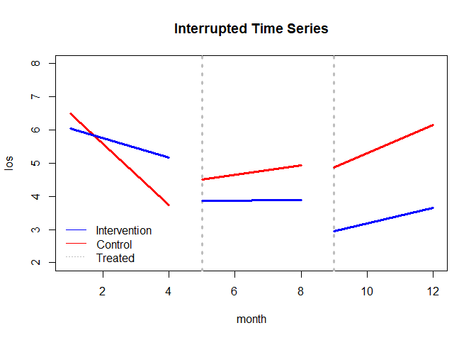
We can also perform an ITS on binary outcomes like death within 30-days. We will examine an intervention and control group at months 5 and 9, which is specified with interrupt= c(5, 9) and its =“two”.
id22 <- assess(formula=death30 ~ ., data=hosprog, intervention = "program",
int.time="month", interrupt= c(5, 9), its="two")summary(id22$ITS)
#>
#> Call:
#> stats::lm(formula = ITS_formula, data = combined_df)
#>
#> Residuals:
#> Min 1Q Median 3Q Max
#> -0.26332 -0.19587 -0.08391 -0.04646 0.95377
#>
#> Coefficients:
#> Estimate Std. Error t value Pr(>|t|)
#> (Intercept) 0.082862 0.075334 1.100 0.2717
#> ITS.Time -0.009101 0.027748 -0.328 0.7430
#> ITS.Int 0.181411 0.110412 1.643 0.1008
#> txi -0.013699 0.039359 -0.348 0.7279
#> post5 0.198078 0.090709 2.184 0.0293 *
#> txp5 -0.026453 0.038946 -0.679 0.4972
#> ixp5 -0.302124 0.126886 -2.381 0.0175 *
#> txip5 0.071580 0.055704 1.285 0.1992
#> post9 0.170102 0.089622 1.898 0.0581 .
#> txp9 -0.014163 0.036857 -0.384 0.7009
#> ixp9 -0.306371 0.133562 -2.294 0.0221 *
#> txip9 0.020050 0.055162 0.363 0.7164
#> ---
#> Signif. codes: 0 '***' 0.001 '**' 0.01 '*' 0.05 '.' 0.1 ' ' 1
#>
#> Residual standard error: 0.334 on 708 degrees of freedom
#> Multiple R-squared: 0.05044, Adjusted R-squared: 0.03569
#> F-statistic: 3.419 on 11 and 708 DF, p-value: 0.0001208interpret(id22)$its
#> Interpretations: ITS
#> --------------------
#> Note: Some variable names below based on time points (or 'interruptions').
#> This analysis is for a two-group, single intervention period (interruption).
#> Positive values indicate higher intervention group values and vice-versa for:
#> post1, txp1, ixp1, txip1, post2, txp2, ixp2, txip2.
#>
#> Intercept is 0.083 and the starting value of the trend for the
#> control group.
#>
#> ITS.Time is -0.009 and the control group's slope prior to intervention.
#> The coefficient is non-significant.
#>
#> ITS.Int is 0.181 and the difference in the level between intervention
#> and control group prior to intervention 1 (intervention - control).
#> The coefficient is non-significant.
#>
#> txi is -0.014 and the difference between the intervention and
#> control group's pre-intervention slopes (intervention - control).
#> The coefficient is non-significant.
#>
#> post5 is 0.198 and the immediate shift in the control group
#> trend line after the 1st intervention start. The coefficient is
#> significant.
#>
#> txp5 is -0.026 and the difference between pre- and post-intervention
#> control group slopes (e.g., change in the pre-intervention
#> slope). The coefficient is non-significant.
#>
#> ixp5 is -0.302 and the difference between the intervention and
#> control groups (intervention - control) in the period immediately
#> after the intervention started (e.g., 1st year of intervention 1).
#> The coefficient is significant.
#>
#> txip5 is 0.072 and non-significant. This is the difference in both
#> group's slope changes since pre-intervention (pre-slopes compared
#> to post-slopes). For example, both have pre-intervention slopes
#> of 2, the control group's slope remained the same, therefore the
#> post 1st intervention slope is 0. And the intervention group's slope
#> increased by 2, then txip1 = 2 (= 2 - 0).
#>
#> post9 is 0.17 and the immediate shift in the control group
#> trend line after the 2nd intervention start. The coefficient is
#> non-significant.
#>
#> txp9 is -0.014 and the difference between 1st and 2nd intervention
#> control group slopes (e.g., change in the 1st intervention
#> slope). The coefficient is non-significant.
#>
#> ixp9 is -0.306 and the difference between the intervention and
#> control groups (intervention - control) in the period immediately
#> after the 2nd intervention started (e.g., 1st year of intervention 2).
#> The coefficient is significant.
#>
#> txip9 is 0.02 and non-significant. This is the difference in both group's
#> slope changes since the 1st intervention (1st intervention slope compared
#> to the 2nd). For example, both have 1st intervention slopes of 2, the control
#> group's slope remained the same, therefore the 2nd intervention slope is 0. And
#> the intervention group's slope increased by 2, then txip2 = 2 (= 2 - 0).
#>
#> Summary 1: For the 1st intervention period, the results show that the
#> intervention group's non-significant shift in death30,
#> post 1st intervention was 0.022. The control group's non-significant
#> shift in death30, post 1st intervention was -0.036. The non-significant
#> difference between both groups is 0.058.
#>
#> Summary 2: For the 2nd intervention period, the results show that the
#> intervention group's non-significant shift in death30,
#> post 2nd intervention was 0.028. The control group's significant
#> shift in death30, post 2nd intervention was -0.05. The significant
#> difference between both groups is 0.078.
#>
#> If there are additional variables in the model then the coefficients
#> above represent effects after controlling for the other variables.The following are corrections of errors and additions in the next version of ham.
Errors corrected are for plot.assess only: 1) DID=“many” time 1 is no longer the intercept and 2) ITS=“two” intercept is now correct.
Additions are for plot.assess only: 1) added some graphing parameters and 2) added arrows and coefficient names to help visualize model coefficients.
Examples of new plotting options are below.
plot(dm1, "DID", add.legend="bottom", ylim=c(2, 8), main="DID: Two No Coefficients", col=c("dodgerblue","magenta"), lwd=7, cex=2, cex.axis=2, cex.lab=1.5, cex.main=3, name=TRUE, )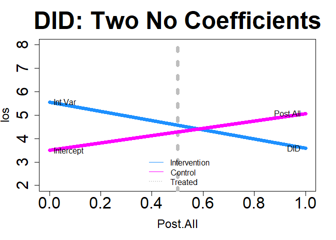
plot(dm1, "DID", add.legend="bottom", xlim=c(-.1, 1.1), ylim=c(2, 8), main="DID: Two", col=c("dodgerblue","magenta"), lwd=7, cex=2, cex.axis=2, cex.lab=1.5, cex.main=3, arrow=TRUE, xshift=c(.02), cex.text=1.5, coefs=TRUE, round.c=2, cfact=T, conf.int=TRUE, adj.alpha=0.2 )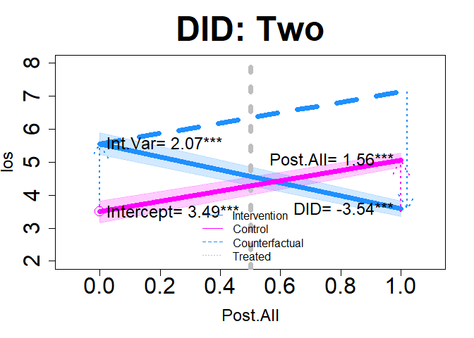
plot(dm2, "DID", add.legend="topleft", xlim=c(-.5, 12), ylim=c(2, 8), main="DID: Many", col=c("purple","green"), lwd=7, cex=3, cex.axis=2, cex.lab=1.5, cex.main=3, arrow=TRUE, xshift=c(.25, .1), cex.text=1.5, coefs=TRUE, round.c=2, cfact=T, conf.int=TRUE, adj.alpha=0.2 )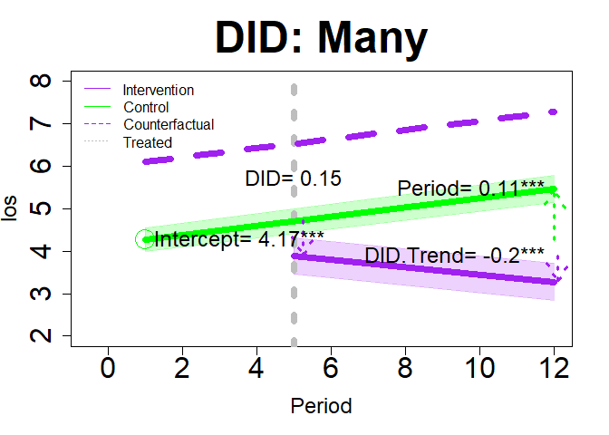
plot(im11, "ITS", add.legend="topleft", xlim=c(-1, 14), ylim=c(2, 8), main="ITS study: SGST", col="thistle", lwd=7, cex=3, cex.axis=2, cex.lab=1.5, cex.main=3, arrow=TRUE, xshift=c(.25, .25), cex.text=1.5, coefs=TRUE, round.c=2, cfact=T, conf.int=TRUE, adj.alpha=0.2 )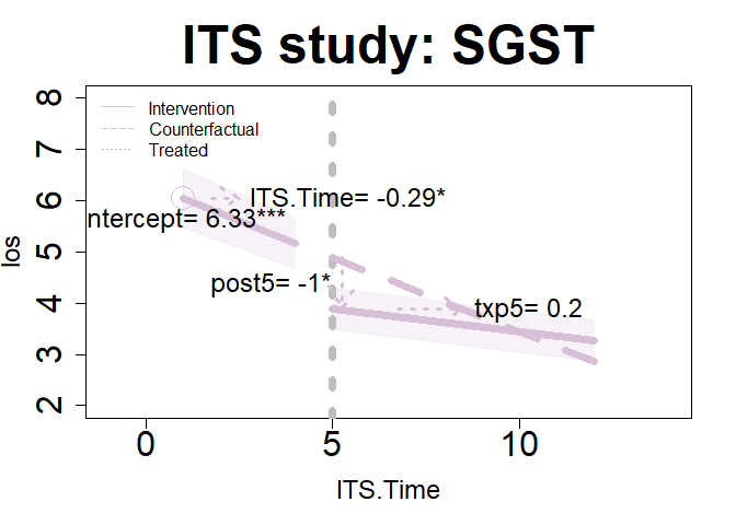
plot(im12, "ITS", add.legend="topleft", xlim=c(-1, 14), ylim=c(2, 8), main="ITS study: SGMT", col="hotpink", lwd=7, cex=3, cex.axis=2, cex.lab=1.5, cex.main=3, arrow=TRUE, xshift=c(.25, .25), cex.text=1.5, coefs=TRUE, round.c=2, cfact=T, conf.int=TRUE, adj.alpha=0.2 )
plot(im21, "ITS", add.legend="top", xlim=c(-1, 14), ylim=c(2, 8), main="ITS study: MGST", col=c("springgreen","salmon"), lwd=7, cex=3, cex.axis=2, cex.lab=1.5, cex.main=3, arrow=TRUE, xshift=c(.25, .25), cex.text=1.5, coefs=TRUE, round.c=2, pos.text= list("post5"=2), conf.int=TRUE, adj.alpha=0.2 )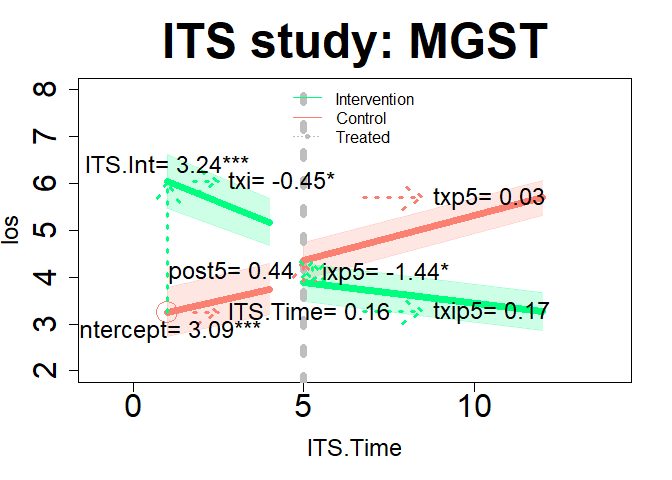
Using all plot options
plot(im22, "ITS", add.legend="top", xlim=c(-.75, 13.1), ylim=c(2, 8), main="ITS study: MGMT", col=c("dodgerblue","goldenrod"), lwd=7, cex=2, cex.axis=2, cex.lab=1.5, cex.main=3, cex.legend=1.25, arrow=TRUE, xshift=c(0, .5), cex.text=1.25, name=F, coefs=TRUE, round.c=2, pos.text= list("txp5"=3, "post9"=4), tcol="springgreen", cfact=T, conf.int=TRUE, adj.alpha=0.3, add.means=TRUE)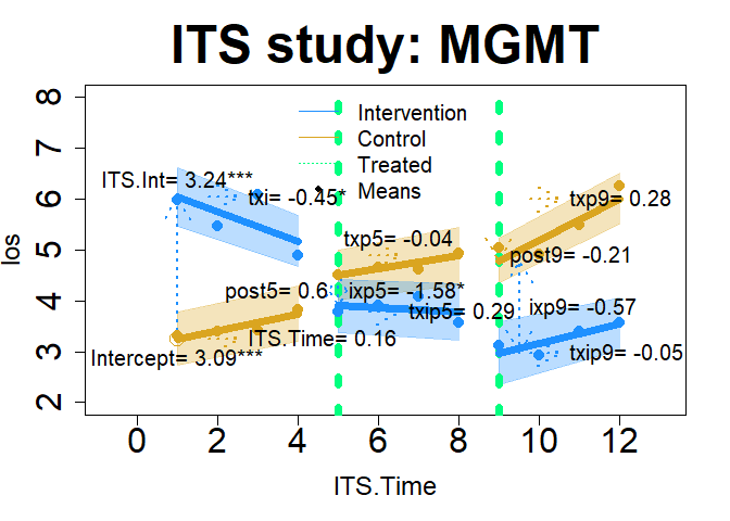
plot(x=gr1, y="roll", lwd=4, gcol=c("red", "blue"), gband=TRUE, overall=TRUE, oband=TRUE, ocol="gray", tcol="green", tgt=4, tpline=c(4,6), tpcol="yellow", name=TRUE, cex.axis=2, cex.lab=2, cex.text=3, cex.main=1.25, adj.alpha=.3)